Model Description
This section provides a brief overview of the models used in the backend of the tool. Each model is designed to address specific tasks related to cluster identification, demand estimation, spatial grid planning, and the optimal sizing of the electricity system. Together, these models contribute to a comprehensive analysis framework supporting the planning and optimization of off-grid energy systems in rural Mozambique. Below is a description of each model and its specific functionality.
- Description of the Clustering Methodology
- Description of the Demand Estimation Model
- Description of the Spatial Grid Optimization Tool
- Description of the Energy System Optimization Tool
Methodology for Clustering Building Centroids to Identify Potential Mini-Grid Sites
Objective
Identify spatially coherent groups of buildings (“communities”) that are promising candidates for mini-grid deployment. The pipeline ingests building centroids and applies density-based clustering (DBSCAN) together with a sequence of geographic filters and post-processing rules that enforce practical siting constraints.
Data Inputs
- Building centroids: latitude/longitude points with attributes such as province, building type, surface area, distance to the existing grid, distance to roads, and island status.
- Existing mini-grids: point locations used to avoid duplicating already electrified or served areas.
- User/analysis parameters:
- min_distance_from_grid (m): the minimum distance from the existing grid (default 20 km)
- min_num_of_consumers: minimum number of buildings required to form a viable cluster
- max_minigrid_network_distance (m): maximum allowable intra-cluster span
- min_distance_to_an_existing_minigrid (m): minimum separation required between a new cluster and an existing mini-grid
- province: the province in which the analysis is conducted
Algorithm Workflow
The workflow begins by querying the database for buildings that satisfy the grid-distance threshold, typically a minimum of 20 km from the existing grid. This threshold is user-settable in the graphical user interface via min_distance_from_grid. The purpose of this criterion is to focus the analysis on settlements where mini-grid solutions are more likely to be relevant than grid extension.
To reflect logistical constraints and accessibility considerations, buildings located on islands are always retained. For mainland areas, buildings that satisfy the grid-distance criterion are retained only if they lie within one kilometer of a road. This pre-screening step ensures that the resulting candidate settlements remain realistically accessible for infrastructure deployment.
The selected centroids are then clustered using the DBSCAN algorithm based on their geographic coordinates. The algorithm uses a default neighborhood radius of 300 meters, derived from empirical observations of settlement morphology in Mozambique, and min_num_of_consumers as the minimum number of buildings required to form a cluster. DBSCAN is particularly suited for this task because it identifies clusters of arbitrary shapes, does not require specifying the number of clusters beforehand, and naturally classifies isolated buildings as noise.
After clustering, a compactness control is applied. For each cluster, the maximum great-circle distance between any two buildings is calculated. Clusters exceeding the threshold defined by max_minigrid_network_distance are discarded because they would imply excessive low-voltage distribution distances and higher network costs. Single-building clusters are also excluded.
Finally, a proximity filter is applied to avoid duplication with existing energy infrastructure. Any cluster whose centroid falls within min_distance_to_an_existing_minigrid of a known mini-grid is removed from the candidate set. This ensures that the model identifies new potential sites rather than settlements already served by existing systems.
Proper parameterization of the clustering process is essential. The neighborhood radius should reflect typical distances between buildings within rural settlements. If the radius is too small, villages may be fragmented into several clusters; if too large, distinct settlements may be merged. The minimum number of consumers represents the smallest viable customer base, while the maximum cluster diameter ensures that resulting mini-grid layouts remain technically and economically feasible.
Description of the Demand Estimation Model
The demand estimation model is designed to simulate electricity demand in rural Mozambique by combining geospatial information, consumer typologies, and stochastic load-profile generation. Its purpose is to estimate settlement-level demand profiles that can be used as direct inputs for mini-grid planning and energy system optimization.
The model distinguishes between three main consumer classes:
- Households (HH)
- Public Services (PS)
- Enterprises
By default, buildings identified in the geospatial dataset are initially classified as households. Public service facilities such as schools, health centers, and administrative buildings can be identified through dedicated geospatial layers and automatically classified as public-service consumers. Users may manually review and adjust these classifications to ensure that local conditions are correctly represented.
Household Demand Categories
Households are categorized into five consumption levels, which serve as proxies for income level, appliance ownership, and energy access:
- Very Low
- Low
- Medium
- High
- Very High
Each category is associated with an indicative daily electricity consumption level expressed in kWh per household per day. These consumption bands also correspond to different appliance bundles and usage patterns. For example, households in the lowest category may primarily use lighting and phone charging, while higher categories may include televisions, refrigerators, fans, and other appliances.
The distribution of these household categories varies depending on the settlement typology. The model distinguishes between rural isolated settlements and rural peri-urban settlements, which typically exhibit different demand structures.
Public Services and Enterprise Loads
Public services and enterprises are represented through predefined consumer categories, each associated with characteristic daily energy consumption and operating schedules.
Examples of public-service consumers include:
- health centers and clinics
- schools and training facilities
- administrative buildings
- police stations
- public lighting
- religious buildings
Enterprise loads represent productive uses of electricity such as:
- retail shops and groceries
- restaurants and bars
- carpentry and metal workshops
- repair shops
- pharmacies
- cybercafés
- agricultural processing equipment
- cold storage facilities
These consumer categories allow the model to capture productive electricity uses that are often important drivers of local economic development in rural electrification projects.
Generation of Load Profiles Using RAMP
Hourly demand profiles are generated using RAMP, an open-source software tool designed for the stochastic simulation of energy demand in contexts where detailed consumption measurements are not available.
RAMP generates load curves by combining information about:
- consumer categories
- appliance ownership
- appliance power ratings
- appliance usage windows during the day
Within the tool, appliance usage is assigned to typical time-of-use patterns such as:
- constant load (24 h)
- daytime usage
- nighttime usage
- morning and evening peaks
- office hours
- workshop operating hours
Using stochastic algorithms, RAMP generates realistic variability in electricity consumption by introducing probabilistic behavior in appliance operation. Instead of producing a single deterministic demand curve, the tool generates demand distributions that better reflect the diversity of real-world consumption patterns.
The resulting hourly demand profiles are aggregated at settlement level and used as direct inputs for the energy system optimization model.
Description of the Spatial Grid Optimization Tool
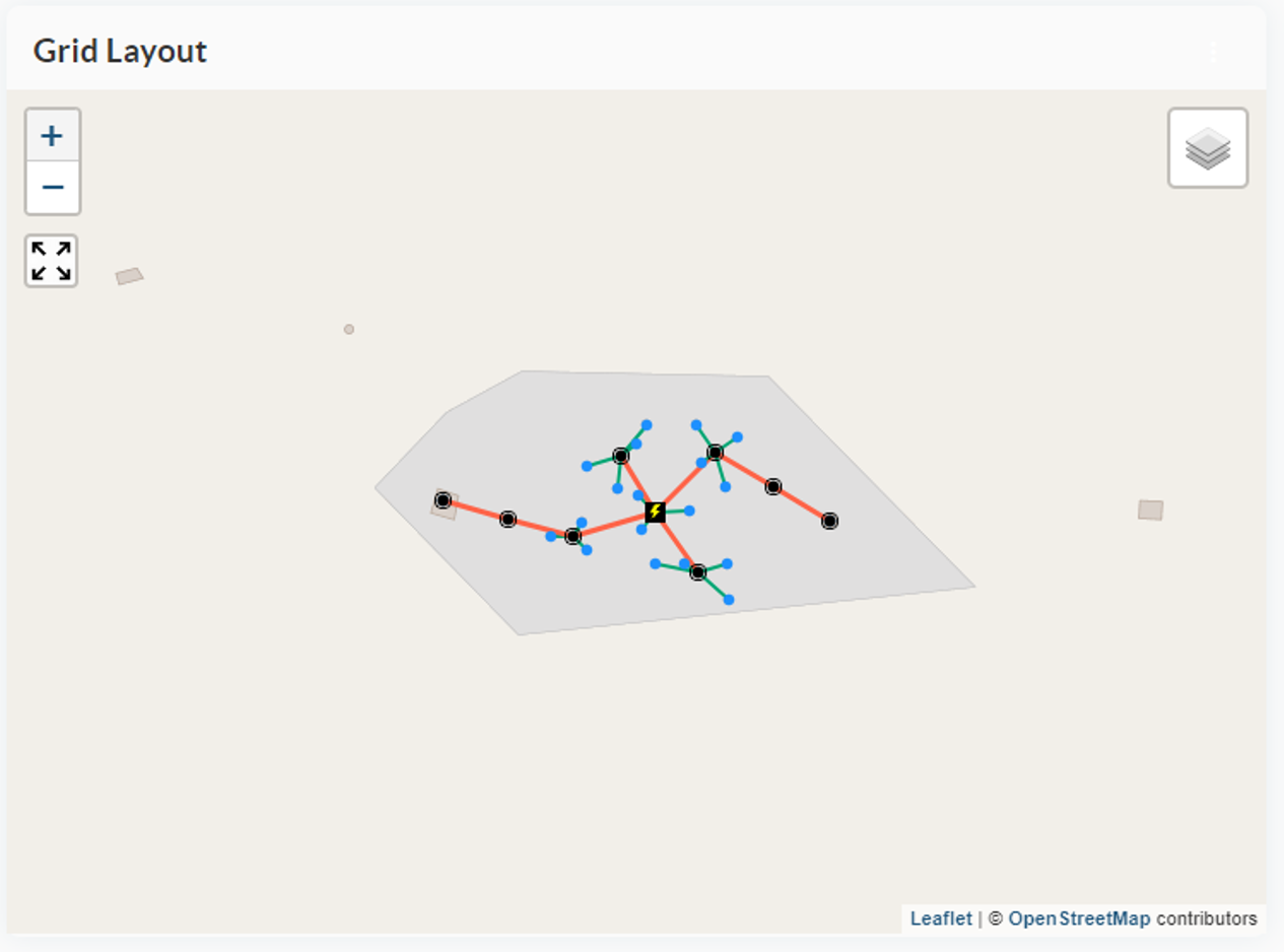
The Spatial Grid Optimization model determines the optimal configuration of the distribution network required to connect consumers within a mini-grid. The objective is to identify the locations of poles, distribution cables, and connection lines that minimize total network distance while satisfying technical constraints.
The starting point of the optimization is the geolocation of individual consumers. Consumers are first grouped using a constrained clustering approach. The centroids of these clusters are used as candidate locations for distribution poles.
Each consumer is connected to its respective cluster pole, forming the initial network structure. The poles are then connected using a minimum spanning tree (MST) algorithm, specifically Kruskal’s algorithm, which identifies the network configuration with the minimum total connection distance.
To ensure practical network layouts, intermediate poles may be introduced where necessary to avoid excessively long cable spans.
The model also includes a mechanism for identifying consumers with particularly high connection costs. In such cases, the user may choose to exclude these consumers from the mini-grid and instead consider alternatives such as solar home systems.
To evaluate this, the costs of poles, connection cables, and distribution lines are allocated among consumers along each branch of the network. The cost allocation begins at the load center, defined as the pole located closest to the median longitude and latitude of the settlement. Consumers are assigned the costs of the infrastructure required to connect them to the load center.
A user-defined parameter called Max Specific Grid Cost defines the maximum acceptable connection cost per consumer. Consumers whose connection costs exceed this threshold may be iteratively removed from the network, starting from the ends of branches. After each removal, the cost allocation is recalculated until all remaining consumers fall below the specified threshold.
- The starting point for the optimization are the respective geolocations of the consumers.

- Clustering of consumers by constrained Kmeans algorithm (size of clusters are limited).

- The centroids of the clusters are taken as the geolocations of the poles.

- Each consumer is connected to its cluster pole.
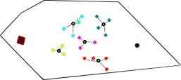
- A minimum spanning tree (MST) is then constructed from this graph, which connects all the poles with minimum total distance (Kruskal's algorithm).
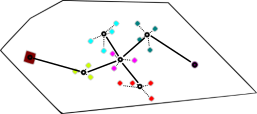
- Addition of intermediate poles to prevent unacceptable cable spans.
Description of the Energy System Optimization Tool
This tool provides a comprehensive framework for designing and optimizing off-grid energy systems that supply electricity to rural settlements. It integrates different generation technologies, including photovoltaic (PV) systems and diesel generators, as well as key components such as battery storage systems, inverters, and rectifiers.
The objective of the model is to determine the most cost-effective system configuration capable of meeting the estimated electricity demand.
Solar resource availability is represented using location-specific datasets and solar modeling tools such as PVLIB, which convert climate data into hourly photovoltaic generation profiles.
Optimization Approach
The system optimization is implemented using oemof.solph, part of the Open Energy Modeling Framework (OEMOF). OEMOF Solph allows flexible representation of energy systems through interconnected components such as energy buses, generators, storage units, and loads.
The optimization problem is formulated as a mixed-integer linear programming (MILP) model. The objective function minimizes the total annualized cost of the energy system.
Annualized costs include:
- capital expenditures for system installation
- operational and maintenance costs
- fuel costs for diesel generators
- replacement costs for components such as batteries
By minimizing total annualized costs, the model identifies the optimal balance between capital investment and operational expenses.
MILP optimization allows the model to represent both continuous variables, such as generation capacity, and discrete investment decisions, such as the installation of additional system components. Although linearization introduces some simplifications compared to nonlinear models, MILP offers a robust balance between computational efficiency and solution accuracy.
System Operation and Unit Commitment
The model also determines the operational dispatch of system components over time. This includes deciding which energy sources should supply electricity at each time step in order to meet demand while minimizing operating costs.
Operational constraints include:
- generator capacity limits
- battery state-of-charge limits
- inverter capacity constraints
- energy balance at each time step
Through this process, the model determines both the optimal system design and the corresponding operational schedule.
Model Outputs
The optimization generates a range of outputs describing both technical and economic system performance.
Key outputs include:
- installed generation and storage capacities
- hourly dispatch time series
- investment costs
- operational costs
- fuel consumption
- estimated CO2 emissions
These outputs provide decision-makers with a comprehensive overview of the expected performance, cost structure, and environmental impact of proposed mini-grid systems.