Model Description

This section provides a brief overview of the models used in the backend of the tool. Each model is designed to address specific tasks related to cluster identification, demand estimation, spatial grid planning, and the optimal sizing of the electricity system. Together, these models contribute to a comprehensive analysis framework, supporting the planning and optimization of off-grid energy systems. Below is a description of each model and its specific functionality.

Description of the Clustering Methodology
Description of the Demand Estimation Model
Description of the Spatial Grid Optimization Tool
Description of the Energy System Optimization Tool

Methodology for Clustering Building Centroids to Identify Potential Mini-Grid Sites

Objective

Identify spatially coherent groups of buildings (“communities”) that are promising candidates for mini-grid deployment. The pipeline ingests building centroids and applies density-based clustering (DBSCAN) together with a sequence of geographic filters and post-processing rules that enforce practical siting constraints.

Data Inputs

Building centroids: latitude/longitude points with attributes (province, building type, surface, distance to existing grid, distance to road, island flag).
Existing mini-grids: point locations used to avoid duplicating already electrified/served areas.
User/analysis parameters:
- min_distance_from_grid (m): the minimum standoff from the existing grid (default 20 km);
- min_num_of_consumers (number of buildings required to form a viable cluster);
- max_minigrid_network_distance (m), the maximum allowable intra-cluster span; and
- min_distance_to_an_existing_minigrid (m), the minimum separation required between a new cluster and an existing mini-grid.
- province, the province in which to conduct the analysis.

Algorithm Workflow

The workflow begins by querying the database for buildings that satisfy the grid-distance threshold, typically a minimum of 20 km from the existing grid. This threshold is user-settable in the GUI via min_distance_from_grid. To reflect accessibility considerations, buildings on islands are always retained due to their distinct logistics. For non-island areas, buildings that already satisfy the grid-distance criterion are kept only if they lie within one kilometer of a road; this pre-screening step yields a concise, realistic set of candidate centroids for settlement-scale electrification.

The preselected centroids are then clustered with DBSCAN on latitude/longitude coordinates. The algorithm uses a default neighborhood radius of 300 meters, a value derived from empirical analysis of existing mini-grids in Mozambique, and min_num_of_consumers as the minimum viable consumer base. DBSCAN’s density-connectivity recovers non-convex, settlement-like shapes, does not require the number of clusters a priori, and naturally labels isolated households as noise. For the fit step, Euclidean distance in geographic degrees is used for efficiency at the spatial scales considered.

Immediately after DBSCAN, the method imposes a compactness control based on geodesic distances. For each provisional cluster, it computes the maximum great-circle distance between any two member points. Clusters whose span exceeds max_minigrid_network_distance are discarded as too dispersed for economical low-voltage distribution, and singleton clusters are also rejected. This post-filter cleanly separates dense, spatially coherent communities from elongated or accidentally bridged aggregates that can appear when density thresholds connect distant hamlets. A final proximity filter prevents overlap with known assets: any cluster whose centroid falls within min_distance_to_an_existing_minigrid of a catalogued mini-grid is excluded. This rule de-duplicates candidates around existing infrastructure and encourages considering network extensions to serve nearby communities.

Parameterization should reflect local morphology and planning assumptions. The neighborhood radius ought to approximate typical inter-building spacing: if set too small it fragments villages; if too large it fuses distinct communities. The minimum sample count encodes the smallest viable consumer base. The diameter threshold provides an orthogonal compactness check: even with adequate density, an excessive spatial span indicates a layout that may be costly to serve. Taken together, these elements yield a transparent, parameter-driven shortlist of mini-grid candidate communities that balances demand concentration, accessibility, and non-overlap with existing systems.

Description of the Demand Estimation Model

The demand modeling tool developed by PeopleSuN aims to predict electricity demand in non-urban Nigerian villages by integrating extensive survey data with the simulation capabilities of the Remote Area Multi-Energy Profiles (RAMP) software. The primary goal of the tool is to model appliance ownership, electricity consumption trends, and the financial capacity of households and enterprises to afford electricity services. By generating detailed consumer profiles based on geographical zones and wealth categories, it provides nuanced predictions of electricity demand to inform off-grid energy planning and implementation.

Survey Data Collection

Quantitative household and enterprise energy surveys (~5,000 total) were conducted, targeting users who already use electricity in some capacity. The survey gathered key data, including:

Average appliance ownership likelihood (%)
Average daily appliance usage duration (minutes)
Appliance power and time of use assumptions (W)
For enterprises and public services: daily opening and closing times, as well as additional "high power energy-intensive appliances"

This data forms the foundation for modeling energy consumption profiles, providing insights into appliance usage patterns, energy demand, and operational characteristics across different user types.

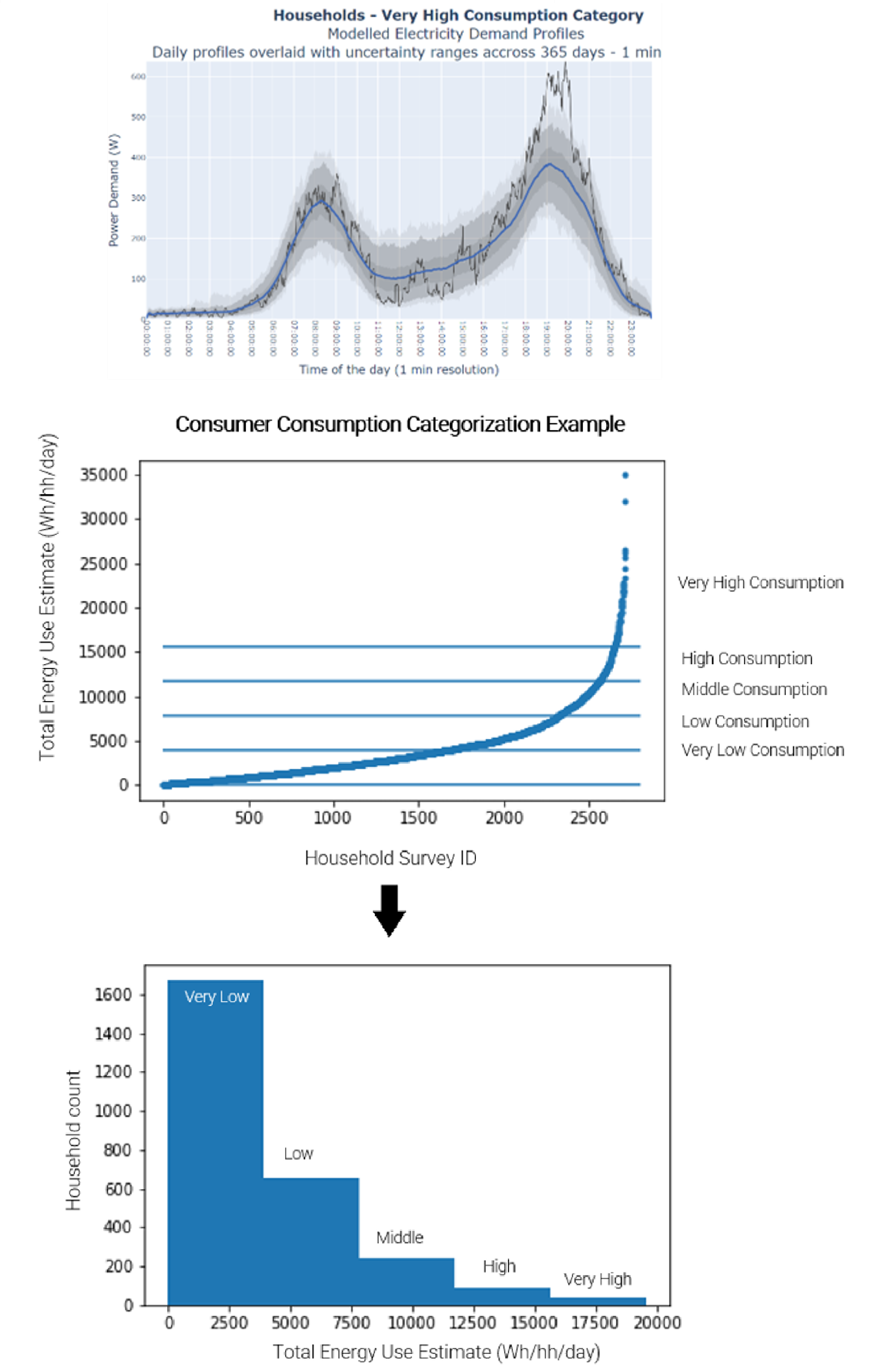
Generating Demand Profiles Using RAMP

The Remote Area Multi-Energy Profiles (RAMP) tool is an open-source software for the stochastic simulation of user-driven energy demand time series. By inputting survey data into RAMP, typical energy consumption profiles for non-urban Nigerian households were developed. The process involved:

Data Analysis and Categorization: Survey data was analyzed to identify patterns in appliance ownership and usage. Households were categorized into consumption levels: Very Low, Low, Medium, High, and Very High, considering factors like appliance types, usage frequency, and household income.
Creation of a National Consumption Profile: A national profile was developed to reflect the diversity of households, accounting for regional variations in wealth, access to energy, and cultural practices.
Simulation with RAMP: The categorized data was used in RAMP to simulate energy consumption patterns, considering hourly, daily, and seasonal variations. Appliance-specific energy use allowed for detailed profiles, including peak demand and load variations.
Stochastic Algorithms: Stochastic methods were applied to account for variability in electricity demand, generating likely distributions of demand rather than fixed values. This enhances the reliability of predictions by considering factors like random appliance breakdowns or changes in usage behavior.

Description of the Spatial Grid Optimization Tool

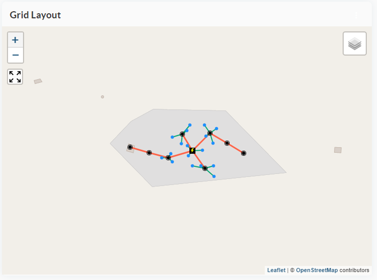
The Spatial Grid Optimization model strategically identifies optimal locations for poles, distribution cables, and connection cables to build the distribution grid. It achieves this by first clustering consumers and then connecting these clusters in a way that results in the lowest total distance. This approach minimizes investment and operational costs while ensuring comprehensive coverage and adherence to connection and distance constraints. Additionally, the model calculates annualized costs for assessing the Levelized Cost of Energy (LCOE).

The model provides the option to identify consumers with particularly high connection costs and exclude them from being connected to the grid. Instead, these consumers should be equipped with a solar home system. To achieve this, the costs for poles, connection, and distribution cables are distributed among consumers along each branch and its sub-branches, starting from the load center of the grid, which is the pole closest to the median longitude and latitude values. For each branch and its sub-branches, the costs are allocated from the load center, with consumers only responsible for the costs of poles and cables connecting them towards the load center. Costs for poles and cables beyond a consumer are borne by subsequent consumers.

The user can set a threshold value called Max Specific Grid Cost. If a consumer exceeds this cost, they are excluded from the grid. Starting from the ends of the branches, consumers with excessive costs are identified, and when consumers are excluded, the cost distribution is recalculated iteratively. The process continues until the consumer at the end of a branch falls below the threshold. Once this happens, the branch is no longer evaluated. The process stops when all consumers at the ends of branches have costs below the threshold.

The starting point for the optimization are the respective geolocations of the consumers.
Clustering of consumers by constrained Kmeans algorithm (size of clusters are limited).
The centroids of the clusters are taken as the geolocations of the poles.
Each consumer is connected to its cluster pole.
A minimum spanning tree (MST) is then constructed from this graph, which connects all the poles with minimum total distance (Kruskal's algorithm).
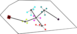
Addition of intermediate poles to prevent unacceptable cable spans.

Description of the Energy System Optimization Tool

This tool is a comprehensive solution for the design and optimization of off-grid energy systems. It integrates a variety of energy sources, including photovoltaic (PV) systems and diesel generators, and supports key components such as battery systems, inverters, and rectifiers. The tool's core functionality lies in its ability to design and optimize these systems to meet specific energy demands in the most cost-efficient way. It uses advanced data modeling techniques, including ERA5 satellite data and PVLIB, to accurately simulate solar potentials, ensuring that PV systems are optimized for the specific environmental conditions of the installation site.

A central aspect of the tool is its focus on minimizing the total annualized costs. Annualized costs account for both the capital expenditures (CapEx) associated with the installation of energy systems and the operational expenditures (OpEx) incurred throughout their lifetime. By optimizing the balance between these costs, the tool generates a configuration that not only meets consumer energy demands but does so in the most financially sustainable manner. This optimization is achieved through mixed-integer linear programming (MILP), a mathematical modeling approach that enables the tool to explore multiple possible configurations and select the one that offers the lowest total annualized cost.

OEMOF-Solph and MILP for Investment Optimization

The tool's optimization relies on the OEMOF (Open Energy Modeling Framework) and its Solph library, which specialize in energy system optimization. OEMOF Solph offers a flexible, open-source platform for modeling various energy converters, storage solutions, and energy flows. Using mixed-integer linear programming (MILP), the tool addresses complex tasks like investment planning and unit commitment.

Investment optimization using MILP offers an efficient approach to system design by minimizing total annualized costs, which include both initial capital investments and ongoing operational expenses. MILP enables the tool to handle discrete decisions, such as selecting additional PV arrays or generators, as well as continuous decisions like determining their optimal capacities. By focusing on a minimal formulation and foregoing the global optimality guarantees of nonlinear programming (NLP), MILP can be solved more efficiently. However, this efficiency comes with the trade-off of accepting some inaccuracies due to the linearization of nonlinear relationships. Nonetheless, MILP provides a practical balance between solution quality and computational performance, making it well-suited for optimizing energy technologies.

Unit commitment refers to the tool's ability to determine which energy units (such as generators or battery systems) should be activated at any given time to meet energy demands efficiently. By using MILP, the tool ensures that these decisions are made in a way that minimizes operational costs, such as fuel consumption and wear-and-tear on equipment, while adhering to technical constraints such as storage capacity and generation limits.

Data-Driven Results for Strategic Decision-Making

The tool generates detailed results regarding the energy system's performance and financial metrics. Key outputs include installed capacities, operational time series, investment costs, CO₂ emissions, and fuel requirements. These results provide stakeholders with a comprehensive overview of the system's operational efficiency and its long-term economic and environmental impacts. This information supports strategic planning for off-grid energy systems across various scales, from small rural electrification projects to larger industrial applications.